One of the major benefits of using Jupyter Books for scientific work is that the narrative and data-processing are part of one and the same work flow. The Jupyter Notebooks, or parts of them, can be directly included in the project - where content is fully shown and accessible on the website but are not present in the printed manuscript. This is done by adding tags to the code cells:
hide-input: results in a dropdown menu on the website where the code can be accessed but removes the code from the printed manuscript
remove-input: removes the input also for the website.
hide-output: hides the output on the website
remove-output: removes the output also on the website.
remove-cell: removes the entire cell from the website and the printed manuscript.
The option to use eval
Below we will cover several common ways of analyzing and presenting data.
Pandas
Source
import pandas as pd
import numpy as np

df = pd.DataFrame(np.random.randn(10, 4), columns=['A', 'B', 'C', 'D'])
df
Output
Matplotlib
import matplotlib.pyplot as plt

plt.figure(figsize=(10, 6))
plt.scatter(df['A'], df['B'], alpha=0.7)
plt.xlabel('Column A')
plt.ylabel('Column B')
plt.title('Scatter Plot of DataFrame Columns')
plt.grid(True, alpha=0.3)
plt.show()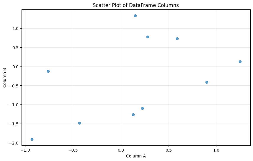
Plotly
import plotly.express as px

fig = px.scatter(df, x='A', y='B', title='Interactive Scatter Plot with Plotly')
fig.update_layout(
    xaxis_title='Column A',
    yaxis_title='Column B',
    showlegend=False
)
fig.show()Altair
import altair as alt

chart = alt.Chart(df.reset_index()).mark_circle().encode(
    x=alt.X('A:Q', title='Column A'),
    y=alt.Y('B:Q', title='Column B'),
    tooltip=['index', 'A', 'B']
).properties(
    title='Interactive Chart with Altair',
    width=400,
    height=300
)

chart
---------------------------------------------------------------------------
ModuleNotFoundError Traceback (most recent call last)
Cell In[4], line 1
----> 1 import altair as alt
2
3 chart = alt.Chart(df.reset_index()).mark_circle().encode(
4 x=alt.X('A:Q', title='Column A'),
ModuleNotFoundError: No module named 'altair'Bokeh
from bokeh.plotting import figure, show
from bokeh.io import output_notebook

# Configure Bokeh to display plots inline
output_notebook()

# Create the plot
p = figure(width=400, height=300, title='Interactive Scatter Plot with Bokeh')
p.scatter(df['A'], df['B'], size=8, alpha=0.7, color='navy')

# Customize the plot
p.xaxis.axis_label = 'Column A'
p.yaxis.axis_label = 'Column B'
p.grid.grid_line_alpha = 0.3

show(p)
Widgets
Source
import numpy as np
import matplotlib.pyplot as plt


x = np.linspace(0,100,10)
y = 2*x+3

plt.figure()
plt.plot(x,y,'k.')
plt.xlabel('x')
plt.ylabel('y')
# plt.savefig('fig1.svg')
plt.show
Figure 1:some caption
Source
inline = 'some text'
second = np.arange(0,5,1)
print(second)
Using eval below to show content / output of the cell above.
Unexecuted inline expression for: inline
Unexecuted inline expression for: second
Source
import numpy as np
import matplotlib.pyplot as plt

x = np.linspace(0,100,10)
y = 2*x+3


fig1, ax = plt.subplots()
ax.plot(x, y, 'k.')
ax.set_xlabel('x')
ax.set_ylabel('y')

fig1.savefig('fig1.svg')
fig1_caption = 'some caption here'
fig1_label = 'fig-no1'
plt.show()
figure below with eval for label and caption.
Figure 2:Unexecuted inline expression for: fig1_caption
Source
import numpy as np
import matplotlib.pyplot as plt
from IPython.display import Markdown

x = np.linspace(0,100,10)
y = 2*x+3


fig2, ax = plt.subplots()
ax.plot(x, y, 'k.')
ax.set_xlabel('x')
ax.set_ylabel('y')

fig2.savefig('fig2.svg')
caption2 = 'some caption here'

display(
    Markdown(
"""
    :::{figure} fig2.svg
    :label: fig-2

    {eval}`caption2`
    :::
"""
    )
)
below there should be a code cell with caption
x = np.linspace(0,100,10)
y = 2*x+3


fig1, ax = plt.subplots()
ax.plot(x, y, 'k.')
ax.set_xlabel('x')
ax.set_ylabel('y')

plt.show()
#| caption: some caption
#| label: some-label
fig2, ax = plt.subplots()
ax.plot(x, y, 'k.')
ax.set_xlabel('x')
ax.set_ylabel('y')
plt.show()
Figure 3:some caption
fig2, ax = plt.subplots()
ax.plot(x, y, 'k.')
ax.set_xlabel('x')
ax.set_ylabel('y')
#| caption: some caption
#| label: some-label
plt.show()