Results - TU Delft's JB Starterkit

With JupyterBook it is possible to make your narrative and data-analysis available in a single file, through Jupyter Notebooks. It is even possible to create interactive materials using widgets on the website, but leave them out in the PDF version (using tags). To run the code below, click the icon in the top right corner. This will connect with a kernel. If the kernel is loaded, click to run the code.

import numpy as np
import matplotlib.pyplot as plt
import ipywidgets as widgets
from ipywidgets import interact
from matplotlib.gridspec import GridSpec

np.random.seed(42)

# Data
x = np.linspace(0, 20, 7)
y = 2.03 * x + np.random.normal(0, 3, len(x))

# range for a
a_min, a_max, steps = 0, 3, 50
a_vals = np.linspace(a_min, a_max, 50)

# make chi-squared curve
chi2_vals = np.array([np.sum((y - a * x)**2) for a in a_vals])
a_opt = a_vals[np.argmin(chi2_vals)]
saved = False # for saving the figure only once

def update(a):
    # Model and residual
    y_model = a * x
    residuen = y - y_model
    chi2 = np.sum(residuen**2)

    fig = plt.figure(figsize=(11, 6))
    gs = GridSpec(2, 2, width_ratios=[2, 1.4], height_ratios=[3, 1], figure=fig)

    ax_main = fig.add_subplot(gs[0, 0])
    ax_res = fig.add_subplot(gs[1, 0], sharex=ax_main)
    ax_chi2 = fig.add_subplot(gs[:, 1])

    # --- upperleft plot: data + model ---
    ax_main.plot(x, y, 'k.', markersize=10, label='Data')
    ax_main.plot(x, y_model, 'r--', linewidth=2, label=fr'Model: $y = {a:.2f}x$')
    ax_main.set_ylabel('y')
    ax_main.set_title('Data and model')
    ax_main.legend()
    ax_main.grid(alpha=0.3)

    # --- bottom left plot: residuals ---
    ax_res.axhline(0, color='gray', linestyle=':', linewidth=1)
    ax_res.plot(x, residuen, 'bo', markersize=7)
    ax_res.vlines(x, 0, residuen, color='b', alpha=0.6)
    ax_res.set_xlabel('x')
    ax_res.set_ylabel('residuals')
    ax_res.set_title('Residuals')
    ax_res.grid(alpha=0.3)

    # --- right plot: chi-squared-curve ---
    ax_chi2.plot(a_vals, chi2_vals, 'k-', linewidth=2)
    ax_chi2.plot(a, chi2, 'ro', markersize=9, label=fr'$\chi^2 = {chi2:.2f}$')
    ax_chi2.axvline(a, color='r', linestyle='--', alpha=0.5)
    ax_chi2.set_xlabel('coefficient a')
    ax_chi2.set_ylabel(r'$\chi^2 = \sum (y - ax)^2$')
    ax_chi2.set_title(r'$\chi^2$ as a function of a')
    ax_chi2.legend()
    ax_chi2.grid(alpha=0.3)

    plt.tight_layout()

    global saved
    if abs(a - a_opt) < (a_max-a_min)/steps and not saved:
        # fig.savefig("figures/chi2_fit.eps")
        # fig.savefig("figures/chi2_fit.png", dpi=450)
        saved = True
    plt.show()

interact(
    update,
    a=widgets.FloatSlider(min=a_min, max=a_max, step=(a_max - a_min) / steps, value=1, description='a')
)

---------------------------------------------------------------------------
ModuleNotFoundError                       Traceback (most recent call last)
Cell In[1], line 3
      1 import numpy as np
      2 import matplotlib.pyplot as plt
----> 3 import ipywidgets as widgets
      4 from ipywidgets import interact
      5 from matplotlib.gridspec import GridSpec

ModuleNotFoundError: No module named 'ipywidgets'

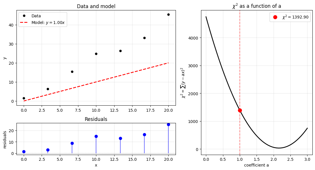
Figure 1 shows the results of fitting our linear model to the data. Parameter $a$ is optimal when the chi-squared curve is at its minimum, which corresponds to the smallest residuals and the best match between model and data.

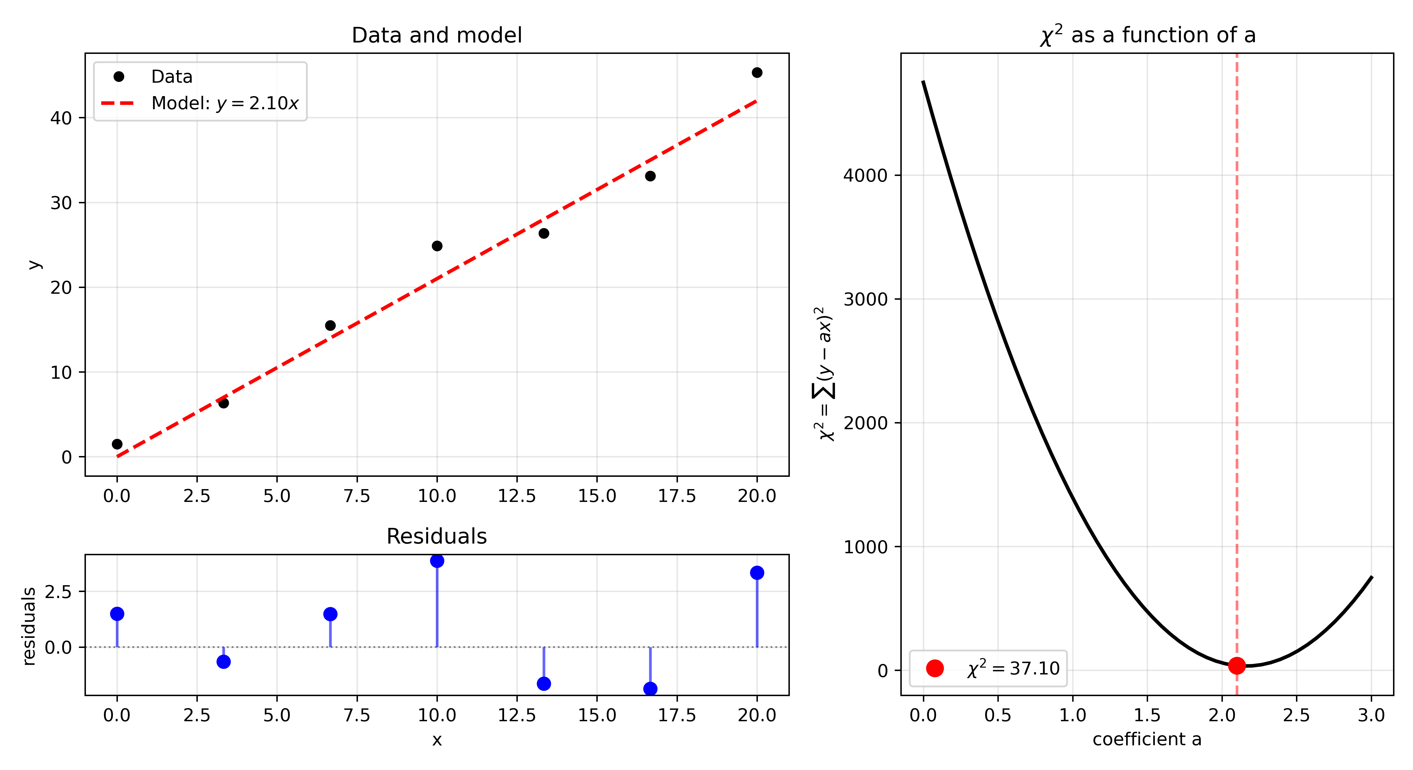
Chi-squared fit, linear trend, with residuals and chi-squared curve. — Figure 1:Fitting our data to a linear model with a single parameter $a$ . The optimal value of $a$ is found when the chi-squared curve (bottom) is at its minimum. The residuals (top right) are smallest at this point, and the model (top left) best matches the data.

5 Results